Reporting your R-script can be done in a matter of seconds by using knitr or R Markdown. These libraries were created to quickly show your R-code as well as results in a wide variety of document types. Knitr can be used to automatically create a report of an existing R-script. R Markdown uses knitr in combination with markdown to create more customised reports.

Knitr
Knitr is ideal to create a report for your colleagues / insiders. It provides the function stitch(), which creates a $\LaTeX$ ( default ) or HTML report of an existing R-script. Apart from the code and results, it also shows the R session information. For more details about this package, refer to the homepage of knitr.
Set-up
Assume we have an R-script called script.R containing just two lines of code.
library(dplyr)
glimpse(mtcars)
The last line will glimpse at dataset mtcars by showing the number of observations, the number of variables and their first values. Further, make sure knitr is installed by running the following command.
install.packages('knitr')
Execution
To quickly generate a report of script.R, simply run the following command.
knitr::stitch('script.R')
The command generated 2 documents in the working directory, namely a $\LaTeX$ file script.tex and a PDF file script.pdf. The PDF-file shows the code, results, R session information and time of execution.
R Markdown
R Markdown is ideal to create a report for your clients / outsiders. It creates a report by writing a markdown document embedded with R code and its results. The document can then be converted to HTML, $\LaTeX$, PDF, Word or even a slideshow. If you are not familiar with markdown, refer to the Markdown article. For more information about R Markdown, refer to the cheat sheet.
In this section, we are going to create an R Markdown document which includes some libraries, glimpses at the dataset mtcars and displays interactive plots.
Set-up
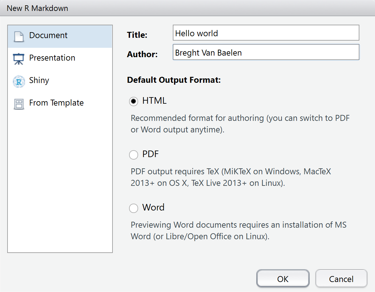
To create R Markdown documents, I highly recommend using RStudio. From RStudio, create a new R Markdown document by clicking File > New File > R Markdown. Specifying the title and author and selecting the desired output format creates an initial YAML-header. The title of this document is set to “Hello world” and the author to “Breght Van Baelen”. Save the document as report.Rmd.

Markdown can be written below the YALM-header and R code can be embedded inline by `r some r-code ` or by a code chunk starting with ```{r} and ending with ``` .
Adding libraries
Add the following text below the YAML-header. What each library is used for will be explained later. Make sure the libraries were downloaded first by using install.packages('the_package').
|
|
Glimpse mtcars
Add the following text to include a glimpse of dataset mtcars to the report. The function kable() produces a markdown output of the table which is then converted to the specified output document.
|
|
Plot datasets
Add runtime: shiny to the YAML-header and the following text to include an interactive plotter to the report. A combobox will be displayed with the option to plot the mtcars or co2 dataset. This will only work when converting to a presentation or a HTML-document and when shiny is running on your localhost. This will be left out when rendering the report. The option echo=FALSE only shows the result and hides the code.
|
|
Execution
The desired output format is specified in the YAML-header. To render report.Rmd, simply press ctrl+shift+k or use the command rmarkdown::render("report.Rmd").
| Output format | Output |
|---|---|
| html_document | html file (webpage) |
| pdf_document | pdf document |
| word_document | Microsoft Word .docx |
| beamer_presentation | beamer slideshow (pdf) |
| ioslides_presentation | ioslides slideshow (html) |
Use the following output format to also keep the $\LaTeX$ document when converting to PDF.
output:
  pdf_document:
    keep_tex: true